Thermoelectric generators (TEG) produce electrical energy from a temperature gradient, but…
- How do I plot the power curve?
- Which voltage range could I extract?
- What would be the minimum temperature difference to generate a determinate voltage (ex. for a cold start-up)?
To answer these questions, a reliable characterization of the TEG module would be needed, because datasheets often are incomplete, or they just do not show the information we need.
In this post, we are going to solve these questions by characterising the TEG.
I will explain which problems I faced and how I turned them around.
Let’s start
Contents
What do we need for a TEG Characterization?
It is a bit tricky to measure or characterise a thermoelectric module. I had troubles at generating a stable and wide temperature difference between both sides.
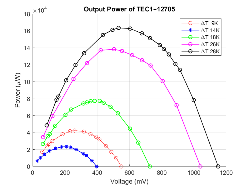
The power curve contains all the data we need to design a system. This is a plot with the the power extracted versus the output voltage of the TEG. But also another graphs like the I-V
Test Bench Set up
A reliable and fixed test characterization test bench must be defined, in order to measure and therefore compare all the TEGs at the same conditions.
Material needed:
- TEG module
- 1 or 2 Heatsinks
- Thermal paste or grease
- A fan or any kind of ventilator
- 2x thermocouples
- 2x multimeters
- Mini clip probe cables
- A sheet of isolator material (I used cork)
- A potentiometer (0-100Ω or 0-500Ω)
- Heat source
Test Bench Construction
TEG modules need a temperature gradient to operate, which means different temperatures between the cold and the hot side. If we have 300ºC on both sides, we will not extract any energy from the module.
If we place the DUT (device under test) over a hot plate, the hot side is going to heat up, but eventually the cold side will do too after some time. So, we will end up with 2 sides at the same temperature. This is like when we fry a steak on the pan, if we wait for minutes, the top side is going to reach hot temperatures and equalize.
To avoid this, we should
- Use a hot side plate are that fits perfectly with the TEG size
- Isolate the hot plate from the cold side
As the first choice is not often possible, I simply isolated the hot and cold sides. I used cork as a thermal isolator, but any other material will also work.
Cut the isolator material to fit exactly the TEG. This material will avoid that the hot flow warms up the cold side and the heatsink.


After placing the TEG module inside the hole, a hot source is necessary for the hot junction and a heatsink for the cold one.
In my case, I use two metal plates to connect thermally the TEG with the hot plate and the heatsink.
To have a good thermal conduction between 2 plates you need to put thermal grease in between
Why?
Apparently, both surfaces are flat and even, but they are not. Even if they are perfectly flat, they have always a surface roughness in the micro-range. So, these micro-air bubbles act as an isolator (because the air is a very good isolator). The air has a thermal conductivity of 0.024 W/m/K when, for example, the copper has 385 W/m/K.
Also, thermal grease is necessary to avoid the presence of air filling the micro-pores in between the TEG and the cupper plates.
Moreover, air bubbles are not desired inside the thermal grease itself. For that, add the paste in the middle and then press both surfaces in order to spread them well.


Electrical connection
The circuit schematic to measure the power and current provided by the TEG, can found in the picture below. The power can be easily calculated following the equation:
P = V·I = V^2 / R = I^2 ·R
The voltmeter should measure directly the two terminals of the TEG, while the ammeter should close the circuit through a potentiometer.
Actually, measuring 2 of the 3 basic electrical magnitudes is enough to estimate the output power. You could measure the resistance and the voltage or current. But in order to measure the resistance, you should unconnect the potentiometer from the circuit… being not so convenient to make a sweep in the resistance.

The value of the variable resistor (potentiometer) can be easily estimated with the expected voltage and power extracted from the datasheet. Or easier: just use a wider potentiometer and then change it if needed. As a rule of thumb, a 500Ω is nice or even 100Ω or 25Ω for smaller commercial TEGs. You can also measure the internal resistance of the TEG to know more or less the range you need.
Heatsinks, natural and forced convection
To increase the temperature gradient, we need to cold down the cold side.
By adding a passive heatsink, we can increase significantly the heat flow from the cold side to the ambient and reducing the cold temperature. This is natural convection heat transfer.
If we add an “unnatural” or “forced” air flow, from a ventilator or any kind of device: it will help even more to reduce the temperature. This will change from the so called natural to forced convention.

By placing the ventilator, align the air direction with the heatsink fins, it will work much better.

The internal resistance of the multimeter
When locking the previous circuit diagram, the internal resistance of the ammeter has to be taken into account when measuring small power TEGs in the range of few mW
To measure small gradient (and therefore small power output) the internal resistance of the measurement device (ammeter) becomes critical.
In the picture below, you can see in red the short circuit point (When you disconnect the potentiometer and short both terminals with the ammeter). This is the minimum power point you can measure with this set-up.
Later, you connect the potentiometer at the starting position with resistance “0Ω”, but they are not really 0, also the cables and so on… So, the second point you can measure is the green one.

The problem arises, when these points are on the right side of the maximum power peak (MPP), as it can be seen below in the example.
In my case, I was measuring the TEG “TEC1 – 12705” with a small 2.2K temperature gradient and using the KeySight U1282A multimeter in µm or mA mode, I would see no maximum point for the TEG as it can be seen on the pic below.


I was testing the various multimeters to see which one perform better.
- Keysight U1282A
- µA mode, very high internal resistance
- A-Mode, better performance
- Fluke 175
- Awful in mA mode
- A mode
- DMM230
- 10A mode more or less
- µA mode no way.
- Agilent 34410A
- Very high internal resistance
On the following test, it was measured with the same conditions using different ammeter devices. It was for a 2.1K temperature gradient.

Concluding, in the range of few mW, the KeySight Multimeter in A mode performs much better in than the other devices, including the Agilent 34410A for characterising TEG modules.

Utilizing a Closed Loop Temperature Control
A better way to measure and characterise the TEGs modules is using, when available, a temperature controller with feedback loop.
The temperature controller heats the plate precisely to a user-defined temperature.
The closed-loop control turns on and off automatically a thermoresistor, which is placed underneath the hot side of the DUT, to adjust the previously defined temperature set point.
The controller has a thermocouple as an input and a voltage output to heat the resistor.
In my case, the controller I used (LakeShore 331 Temperature Controller) has 2 temperature inputs: Probe A for the hot plate with the loop control and probe B for the cold side of the DUT. Therefore, the gradient can be very easily monitored.

To adjust the setpoint just press the button 6 (Setpoint) and then introduce the new value.
Power Curve Calculation
A power or a current curve can be drawn for each given temperature gradient.
To measure the current curve for a fixed temperature gradient, the impedance of the circuit must be modified. For this simple circuit, modifying the potentiometer value you will get a current point.
Then the power curve can be post-calculated from the current by the well-known formula P=V·I
To calculate and plot the power and V-I curves, you can use the basic template I updated to this link: misCircuitos.com/TEG_template
In the template, you can use a single Excel page for each temperature gradient or use a single matrix for all the temperatures adding an extra column. I recomend the single matrix version, as it is going to be much easier for the post-processing and plot

Matlab Postprocess
Excel curves are fine for a first preview, but maths software like Matlab or Octave will give you more possibilities to create nicer and representative plots.
Also, Excel has troubles at plotting several graphs together in the same plot when the X-axis coordinates for the multiple lines does not match.
Matlab is way better for plotting complex graphs
To ease the process, the following Matlab script generates automatically the plots and save them in the path folder as a png picture.
Two versions were programmed: One with one matrix for each temperature gradient and the second version with one single matrix with all the data.
Version 1.0
The measured data has to be imported conveniently in matrixes with 3 columns:
voltage; current; power;
The name for each matrix is given as “a”, “b”, “c”, etcetera, bus this can be modified at any time.
Version 2.0
A big matrix with, at least, 4 columns is given as a parameter to the Matlab function.
Voltage;current;Power;Gradient;
The function has three parameters: matrix with the data, name of the device or test, save (1 or 0).
The matrix of data is mandatory to be filled, but the other 2 are optional. The default value for the name is ‘TEG’ and by default is disabled the automatically save of the plots.
Three options to plot the data:
% example of use
>> plotTEG(data)

% example of use with the name of the device for the graphs
>> plotTEG(flex,'-12705')

% example of use with name of device and save ON
>> plotTEG(flex, '-12705',1)
The output of the function is the following three graphs:


Temperature-Voltage plot Control
This plot is useful to control and determine how precise was the temperature adjustment during all the characterization.
If you plot the temperature gradient versus the open-circuit voltage of each gradient, you should get something like the pic above. Then you plot a linear regression with those points.
The closer to zero and less dispersion, the better
If we could measure very small gradient and power, when the temperature gradient tends to zero, the open-voltage circuit should also do. By this way, making a linear regression to estimate where the zero-cross point is, we can say how well the measure in general was.
This following graph have more dispersion than the previous one, so we can conclude that we have a less acurate results.

Verilog Model
A verilog model can be created from a lock up table to simulate the behaviour of a specific physical device inside a simulation environment like Cadence or another tool.
For more info on how to create your own verilog model based on a look up table: misCircuitos.com/verilog-model
Matalb code version 1.0
%{
Plot a TEG characterization curve with multiple temperature gradient

Each temperature gradient value have a matrix with 3 columns: voltage, Current
and Power

Version: 1.0
Date: Feb 2020
Autor: Alberto Lopez
Contact: AlbertoLopez@AlbertoLopez.eu
  %}

%% Power-curve
figure(1)

grid on;
hold on;

plot(b(:,1),b(:,3),"o-r");
plot(a(:,1),a(:,3),"*-b", "linewidth", 1);
plot(c(:,1),c(:,3),"o-g", "linewidth", 1);
plot(d(:,1),d(:,3),"o-m","linewidth", 1);


%set(gca, "linewidth", 3, "fontsize", 25)
title("Output Power of CP105433H");
xlabel ( "Voltage (mV)");
ylabel ("Power (\muW)");
legend ("\DeltaT  6K", "\DeltaT 11K","\DeltaT 19K", "\DeltaT 22K", "location", "northeast");

%save the plot automatically. Comment this line to avoid overwriting it
saveas (1, "Power-thermo-CP105433H.png");


%% V-I curve
figure(2)
grid on;
hold on;

plot(b(:,1),b(:,2),"o-r","linewidth", 2);
plot(a(:,1),a(:,2),"*-b", "linewidth", 2);
plot(c(:,1),c(:,2),"o-g", "linewidth", 2);
plot(d(:,1),d(:,2),"o-m","linewidth", 2);


title("V-I curve of CP105433H");
xlabel ( "Voltage (mV)");
ylabel ("Power (\muW)");
legend ("\DeltaT  6K", "\DeltaT 11K","\DeltaT 19K", "\DeltaT 22K", "location", "best");

%save the plot automatically. Comment this line to avoid overwriting it
saveas (2, "I-V-thermo-CP105433H.png");
Matlab code Version 2.0
function plotTEG(data, device, save)
 %{
Plot a TEG characterization curve with multiple temperature gradient

Each temperature gradient value have a matrix with 4 columns: voltage,
Current, Power and temperature Gradient

Version: 2.0
Date: Feb 2020
Autor: Alberto Lopez
Contact: AlbertoLopez@AlbertoLopez.eu
  %}
mat = data;
%% DEFINES
DEVICE = '-TEG';
SAVE = 0;
if nargin == 2
  DEVICE = device;
elseif nargin == 3
    DEVICE = device;
    SAVE = save;
end
%default values for not define parameters

%% Limit Calculation

%First calculate the section where the same temperature gradient applies
temp = mat(1,4); %start with the first gradient
limits(1) = 1;  %initializate the limit vector to store where the temperature gradients changes
j= 2;
for i =1:1:length(mat)
    if mat(i,4)~=temp;
        limits(j)=i;
        j= j+1;
        temp = mat(i,4); %asign the new value for the reference
    end

end
limits(j) = length(mat)+1; %store the last value
% Now Ploting can be started

%% Power Curve
figure(1)

grid on;
hold on;

for i=1:1:length(limits)-1
    plot(mat(limits(i):limits(i+1)-1,1),mat(limits(i):limits(i+1)-1,3),"o-");
end


% Power Figure Stetics
title(['Output Power of ', DEVICE]);
xlabel ( "Voltage (mV)");
ylabel ("Power (\muW)");

% Generate the legend
str = {strcat('\DeltaT = ' , num2str(mat(1,4)), 'K')};
for i=2:1:length(limits)-1
    str = [str , strcat('\DeltaT = ' , num2str(mat(limits(i),4)), 'K')]; % after 2nd loop
end
legend(str{:}, "location", "best");

% Give a name to the title bar.
set(gcf, 'Name', 'Power Plot- Alberto Lopez', 'NumberTitle', 'Off')
% Enlarge figure to full screen.
set(gcf, 'Units', 'Normalized', 'OuterPosition', [0 0 1 1]);
%save the plot automatically when SAVE = 1
if SAVE saveas (1, [DEVICE,'-Power-curve-TEG','.png']); end

%% voltage-current curve
figure(2)

grid on;
hold on;

for i=1:1:length(limits)-1
    plot(mat(limits(i):limits(i+1)-1,1),mat(limits(i):limits(i+1)-1,2),"o-");
end

% Power Figure Stetics
title(['Voltage-Current of ', DEVICE]);
xlabel ( "Voltage (mV)");
ylabel ("Current (\muA)");

% Generate the legend
str = {strcat('\DeltaT = ' , num2str(mat(1,4)), 'K')};
for i=2:1:length(limits)-1
    str = [str , strcat('\DeltaT = ' , num2str(mat(limits(i),4)), 'K')]; % after 2nd loop
end
legend(str{:}, "location", "best");

% Enlarge figure to full screen.
set(gcf, 'Units', 'Normalized', 'OuterPosition', [0 0 1 1]);
% Give a name to the title bar.
set(gcf, 'Name', 'V-I Plot- Alberto Lopez', 'NumberTitle', 'Off')
%save the plot automatically when SAVE = 1
if SAVE saveas (2, [DEVICE,'-V-I-curve-TEG','.png']); end

%% Voltage-Temperature
figure(3)

grid on;
hold on;
clear x y;
x= 99;
y =1999;
for i=1:1:length(mat)
    if mat(i,2) == 0
        x = [x,mat(i,4)];
        y = [y,mat(i,1)];
        %plot(mat(i,4),mat(i,1),"o-");
    end
end
x(1)=[]; %delete the first element of x vector
y(1)=[];
%curve fit
p = polyfit(x,y,1);
x1 = linspace(0, max(mat(:,4)), 50);
y1 = polyval(p,x1);

plot(x, y, 'ro', 'MarkerSize', 4, 'LineWidth', 3);
plot(x1, y1, '-', 'LineWidth', 2)
text(0,y1(1),['\leftarrow ', num2str(y1(1))])


%  Figure Stetics
title(['Temperature-Voltage of ', DEVICE]);
xlabel ( "Temperature (ºC)");
ylabel ("Open Circuit Voltage (mV)");
%set axis limits to show the zero
xlim([0 inf])
ylim([y1(1)*2 inf])

% Give a name to the title bar.
set(gcf, 'Name', 'Temperature-Voltage Plot- Alberto Lopez', 'NumberTitle', 'Off')
%save the plot automatically when SAVE = 1
if SAVE saveas (3, [DEVICE, '-T-Voc-curve-TEG','.png']); end

end %end function
I hope this article was helpful and interesting for you. If you may have any questions, please write them down in the comments below


Good morning Alberto, I want to use a Peltier element (or TEG, which is the same as I understand) as a calorimeter to measure the 3mm beam diameter light output of (diode) lasers in the 1-100 mW range. So, therefore I’m interested in obtaining as much as Open-Circuit-Voltage (Voc) possible per absorbed laser light heating input power (= per delta-T on the TEG). So, I,m not interested in output current (I=0) or output power (P=0) but only in the highest Voc.
Therefore I have some questions:
1. should I use (in principle) a larger (40×40 mm2) or a smaller (e.g. 10×10 mm2) TEG and why larger or smaller ? The laser beam is 3 mm diameter only.
2. should the TEG (in principle) have a higher (appr. 4 Ohms) or a lower (appr. 2 Ohms) internal resistance, and why or why not ?
3. should I use a single or a stacked TEG, and why or why not ?
4. I could not figure out how the TEG-surrounding cork insulator plate could actively help preventing the TEG-cold-side from heating up, because the cork is only replacing air in a position where there is no themal radiation that could heat the other/co;der TEG-side up ? I can imagine that filling up the empty space between the hold and cold TEG-sides around the semiconductor pillars could help preventing heating up.
5. any other advice wih respect to optimize my laser output (calory) optical power meter would be helpful.
I’m looking very much forward to your reaction.
Thank you in avance. Best regards, Guus Möhlmann (The Netherland)
Thank you for the informative article.
I was wondering why the power output drops at higher voltages? I assume you’d want to operate your TEG at the maximum value?
Hello Matthew,
Yes, this phenomenon occurs also in solar cells or other generation devices. The current drops quasi linearly with the voltage… so making the multiplication for obtain the power, we get this characteristic power curve.
To operate TEG or solar cells at higher voltages, charge pumps are normally used in energy harvesters, which is the topic of my phD thesis.
Hope I could help you more.
Best Regars. Alberto
I am also confused about the power calculation. Is the calculation for P = V^2/R, open circuit voltage and internal resistance? I cannot make use of laboratory equipment at the moment, so I’m hoping to be able to calculate the power from home after calculating a rough value for internal resistance and using voltage from my COMSOL simulation. I’m struggling to get either current or resistance from my simulation so calculating by hand a rough value is my first approach.
Ciao Alberto
Many thanks to share your knowledge and tips
I have a small youtube channel , to share some knowledge too or just too share how to build toys
I just built a setup for teg measurement yesterday,
I m measuring 3 sp1848 27145 sa modules
Cheap one from aliexpress
I would like to review it in order to let the people know if they can start playing harvesting for cheap
The open load voltage is as specified 1,8v@40deg diff
About the current they claim 368mA ‘generating current’ but they don t specify at which load
I measured 282mA @0,86v
Is it ok?
Where do i find the i v curv for this module? (Even from other brand)
Thanks Fabio
Hello Fabio!
Nice niche of your youtube channel 🙂
TO obtain the I-V curve, you must change the load with a potentiometer, like in this picture: Variable resistor schematic
The measure of 282mA @0,86v is only one point, you must calculate several of them to get the I-V curve… but you are on the right way!
I am curious… How do you get the 40ºC of difference??
Best Regards
Alberto
Thanks for the reply
And sorry for the late reading
I have a kind of stable setup
with on the bottom side a big heat sink with an hole for the thermocouple immersed in a large pot of water, and in the upper hot side a 5mm alu plate, with small hole in the middle for thermocouple. And with 2 x50w resistor.
I keep constant temp adjusting(manually) the power on the resistors.
When i draw more current probably the conducibility of the peltier module is changing so i have to adjust the power on the resistors and wait to stabilize.
Still is not clear
The teg seller site claims:
Thermoelectric EMF (a): >190×μV/℃
Electrical conductivity (σ): 850~1250Ω-1.cm-1
Thermal conductivity (K): 15~16×10-3-W/℃cm
Good value(Z): 2.5~3.0×10⁻³W/℃
Size: 40x40x3.6mm.
Temperature difference of 20 degrees: open circuit voltage 0.97V, generating current: 225MA.
Temperature difference of 40 degrees: open circuit voltage 1.8V, generating current: 368MA.
Temperature difference of 60 degrees: open circuit voltage 2.4V, generating current: 469MA.
But my question is:
What does it mean generating current?
Is it the short circuit current?or the mpp current?
Thanks
Fabio
Ps the niche channel is called “Maker Fabio”
Hi Fabio,
I am also stuck at the point how we find the load resistor. Do you find the answer, please share with me.
Hello Alberto
Could you kindly advice on the characterization of a TEG performance (eg, Power Output) through the measurement of Current and Voltage, while there is no load (eg resistor or potentiometer) connected to it. This is not necessarily to plot the Power curve but to have a realistic idea about the performance, even if you were to vary the temperature difference. How crucial is the load when characterizing the TEG?
Hello Alex,
yes, if you only measure the open-circuit voltage, you have an average output power of zero. With this you can not estimate the real output power of the TEG, so far I know.
Best Regards
Hey Alberto,
How can I find the load resistor to actually calculate the generated power from Teg Cell. As I am using 10W Resistor vary from 0-1000 ohm, but I can’t find the maximum point. Please guide me, I am stuck at this point.
Hello,
You can measure the internal resistor of the TEG at that specific operating point (temperature gradient) to have an idea of the order of the resistance.
Sometimes, when the power is so little, the internal resistance of the ammeter and the power taken by the voltmeter affects a lot and you can only see the rising up curve and not the maximum point.
What kind of curve do you get when you sweep the R? what about the ammeter and voltmeter? the temperature gradient?
Regards
Alberto
Bonjour
Est ce que cette technique (TEG) peut etre industrielle
c.a.d si on multiplie les modules, avec une difference de temperature constante de 50°, et qu’elle ordre de grandeur de courant peut etre récupérer.
Marci d’avance.
Bonjour,
Sorry, Je ne parle français
Regards
Alberto
Thanks for excellent info I was looking for this information for my task.