The Miller transformation is a powerful technique for simplifying and analyzing of circuits by inspection.
Miller transformation simplifies CMOS circuits by replacing the feedback capacitor with 2 grounded capacitors, whose values depend on the gain of the circuit and the original feedback capacitance.
The Miller theorem transforms an impedance between two nodes into two separate impedances referred to ground, without changing the circuit behavior or node voltages.
Contents
Miller Effect: General Rule
The Miller theorem redefines and transforms a floating impedance, connected to 2 nodes (labeled as 1 and 2), into 2 new impedances referred to ground at each node.
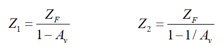
The resulting impedances are expressed as a function of Av, the gain from node 1 to 2. For more details about the equations, refer to the Miller theorem.
This transformation is also called “Miller Multiplication” when used to multiply the apparent value of a capacitance, especially in feedback “Miller” compensation networks. Therefore, the silicon area of the capacitor is reduced by Av factor.
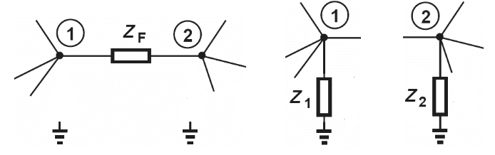
From the floating impedance two new impedances are created, whose value are:
Limitations
This Miller Effect can help us to solve complex circuits by simplifying floating impedances or capacitors and referring them to ground. However, there are several limitations or drawbacks!!!
The Miller’s equations described above cannot be used with complete accuracy. This is because the gain (Av) varies with the frequency.
The gain is typically assumed to be the low-frequency or DC gain (Ao), even though the gain is inherently a function of frequency.
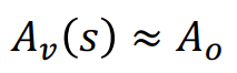
Therefore, when we use this formula, it is called “Miller Approximation”, which is sufficient for most of the cases.
The feedforward zero is lost after the Miller transformation. The zero must be calculated and taken into account before applying the Miller modifications.
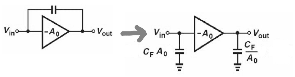
Miller Transformation with Capacitors Only
The most common case of the Miller effect involves pure capacitors.
In the generic case, a feedback capacitor Cf, as shown in the following schematic, can be separated into two equivalent grounded capacitors using the Miller multiplication.
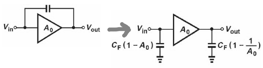
For relatively high gains (Av>> 1) the Miller impedances are simplified to:
Examples of Miller Effect
Let’s clarify the Miller transformation with some practical examples.
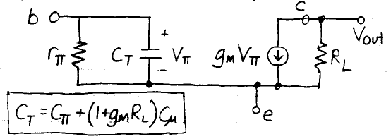
Bipolar Common Emitter
Although, it is not shown in the schematic, the base-collector capacitance is implicit in it.
The calculation of the input capacitance of the common emitter stage with a resistive load at high frequencies is not trivial and needs from the aforementioned Miller transformation.
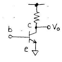
First, we draw the small-signal model, including the stray base-collector capacitance:
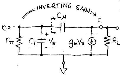
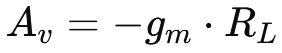
The gain of the circuit from the input (base) to the output (collector) is Av = -gm·RL
Rearranging the small-signal circuit by applying the Miller transformation, the C𝛍 capacitor is “Miller multiplied” by (1-Av) and now appears in parallel with Cπ.
The common emitter equivalent model, rearranging the capacitor C𝜇, can be expressed as:
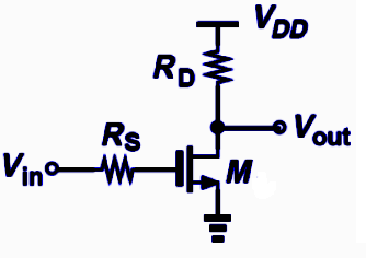
MOSFET Common Stage
Similar to the previous example, but using CMOS technologies. In this case, we are going to analyze a Common Stage including the gate-drain capacitance. The dc gain is Av= -gmRd, considering ro infinite.
The small-signal equivalent circuit:
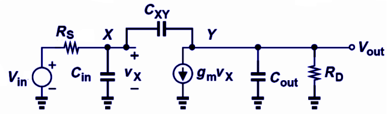
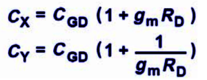
Splitting the capacitor Cxy into 2 capacitors applying the Miller transformation
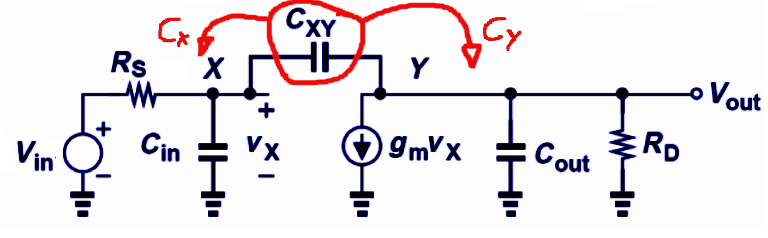
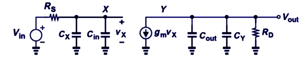
The new capacitors referred to ground and attached to the X and Y nodes are:
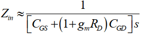
Common Source Stage
The input impedance of a CS stage includes a “not-referred to AC ground” capacitor, which may be converted through the Miller Effect.
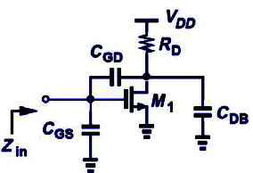
The corresponding input capacitance and impedance are:
![]()
As you can see, the Miller transformation is a valuable tool for simplifying circuit analysis by converting floating impedances, especially capacitors. Nonetheless, the Miller effect is exploited for STB compensation, being widely used in multistage op amps as an effective method to improve its frequency behavior.


